Example Notebook

Example Notebook¶

Authors:

**Edom Moges¹, Ben Ruddell², Liang Zhang¹, Jessica Driscoll³, Parker Norton³, Fernando Perez¹, and Laurel Larsen¹ **

¹ University of California, Berkeley

² Northern Arizona University

³ United States Geological Survey

Environmental Sytems Dynamics Laboratory (ESDL) University of California, Berkeley

 ==================================================================================
 --------------------***********************************************---------------
 ==================================================================================

1 HydroBench: Hydrological Model Benchmarking and Diagnostics
2 Load Libraries
3 Load the watershed observed and model data
4 Predictive (statistical) model performance metrics
- 4.1 Hydrograph and Statistical metrics
- 4.2 Summary table of predictive performances
5 Hydrological Signature based Model Diagnostics
6 Information theoretic based model benchmarking
- 6.1 Executing the info-flow code for the watershed
- 6.2 Interpreting the MI and TE results for model diagnostics
  - 6.2.1 Tradeoff between functional and predictive model performances
  - 6.2.2 Process Network plots

Introduction¶

Hydrological model performances are commonly evaluated based on different statistical metrics e.g., the Nash Sutcliffe coefficient (NSE). However, these metrics do not reveal neither the hydrological consistency of the model nor the model’s functional performances, such as how different flux and store variables interact within the model. As such, they are poor in model diagnostics and fail to indicate whether the model is right for the right reason. In contrast, hydrological process signatures and information theoretic metrics are capable of revealing the hydrological consistency of the model prediction and model internal functions respectively. In this notebook, we demonstrate the use of interactive and reproducible comprehensive model benchmarking and diagnostic using:

a set of statistical predictive performance metrics: Nash Sutcliffe coefficient, Kling and Gupta coefficient, percent bias and pearson correlation coefficient
a set of hydrological process based signatures: flow duration curve, recession curve, time-linked flow duration curve, and runoff coefficient, and
information theoretic based metrics, particularly Transfer Entropy (TE) and Mutual Information(MI).

We demonstrate the application of these metrics on the the National Hydrologic Model product using the PRMS model (NHM-PRMs). NHM-PRMS has two model products covering the CONUS - the calibrated and uncalibrated model products. Out of the CONUS wide NHM-PRMS products, this notebook focused on the NHM-PRMS product at the Cedar River, WA.

Notebook description¶

This notebook has four steps:

Loading the calibrated and uncalibrated NHM-PRMS model product (Section 3)
Interactively evaluating model performances using predictive performance metrics (Section 4)
Diagnosing model performance using hydrological process signatures (Section 5),
Executing information theoretic based model performance evaluation to understand (Section 6):

i. tradeoffs between predictive and function model performance (Section 6.2) ii. model internal function using process network plots of Tranfer Entropy (Section 6.3)

Acknowledgements¶

This work is supported by the NSF Earth Cube Program under awards 1928406 and 1928374, the Moore Foundation and the Powell Center USGS.

Load Libraries¶

%matplotlib inline
import pandas as pd
import numpy as np
import datetime as dt
import matplotlib.pyplot as plt
from tqdm import tqdm
import copy
import os
import glob
import matplotlib.colors as colors
import matplotlib.cm as cmx
from matplotlib.lines import Line2D
import ipywidgets
from ipywidgets import fixed
from termcolor import colored
from scipy import interpolate


import sys
import time
import random
import os
import math
import pickle
from matplotlib import cm

import xarray as xr
import numcodecs
import zarr

from joblib import Parallel, delayed

from pandas.plotting import register_matplotlib_converters
from matplotlib import rcParams
rcParams["font.size"]=14
plt.rcParams.update({'figure.max_open_warning': 0})
register_matplotlib_converters()

import holoviews as hv
from holoviews import opts, dim
from bokeh.plotting import show, output_file
hv.extension("bokeh", "matplotlib")

## Local function
sys.path.insert(1, './Functions')

from PN1_5_RoutineSource import *
from ProcessNetwork1_5MainRoutine_sourceCode import *
from plottingUtilities_Widget import *

# local file paths
np.random.seed(50)
pathData = (r"./Data/")
pathResult = (r"./Result/")

Load the watershed observed and model data¶

This notebook uses a specific standard data input format. The standard data input format is a tab delimited .txt file. The column names are specified in the following cell.

In order to apply to a different dataset, please adopt and follow the standard data format.

Two products of the NHM-PRMS are loaded:

the calibrated NHM-PRMS model product - in this model version, the model parameters are mathematically optimized.
the uncalibrated NHM-PRMS model product - in this model version, the model parameters are estimated based on their physical interpretation.

FName = [12115000]# Additional NHM-PRMS USGS stations:[10296000, 1105600, 12414900, 14141500, 2482550, 13340600]
k = 0
nameFCalib = str(FName[k]) +'_Calibrated.statVar' 
nameFunCalib =  str(FName[k]) +'_unCalibrated.statVar' 

# NHM PRMS simulation results names - TableHeader
TableHeader = ['observed_Q','basin_ppt','basin_tmin','basin_tmax','model_Q','basin_soil_moist','basin_snowmelt','basin_actet','basin_potet']
# Calibrated model
CalibMat = np.loadtxt(pathData+ nameFCalib, delimiter='\t') # cross validate with matlab
#CalibMat[0:5,:]

# Uncalibrated model
UnCalibMat = np.loadtxt(pathData+ nameFunCalib, delimiter='\t') # cross validate with matlab
#UnCalibMat[0:5,:]

startD = '1980-10-01'
endD = '2016-09-30'
dateTimeD = pd.date_range(start=startD, end=endD)
#plt.plot(dateTimeD, CalibMat[:,0])

Predictive (statistical) model performance metrics¶

This section demonstrates model evaluation based on the most common hydrological model predictive performance measures- the Nash Sutcliffe coefficient (NSE), Kling-gupta (KGE), Percent Bias (PBIAS) and Pearson Correlation Coefficient. Two versions of these metrics are adopted - the untransformed and their log trasformed version. These two metrics are suited to evaluate model predictive perormance in capturing the different segments of a hydrograph. For instance,

Untransformed Nash-Sutcliffe coefficeint (NSE) - as an L2-norm, NSE is biased towards high flow predictive performance. This makes NSE suited for evaluating model’s performance in capturing high flows.
Log transformed Nash-Sutcliffe coefficeint (logNSE) - biased towards predictive performance of low flows. This makes logNSE suited for evaluating models’s performance in capturing low flows.

Interactive widgets are used to reveal the comparative performance of the calibrated and uncalibrated model performance using the above two common predictive performance measures.

Hydrograph and Statistical metrics¶

The ipywidges below demonstrates the use of interactive computation particularly to a two version model. It can easily be adopted to a model with multiple model versions.

The main function is in this ipywidgets is PredictivePerformance(.). It has inputs of:

nameFCalib - the calibrated model table
nameFunCalib - the uncalibrated model table
obsQCol and modQCol - column identifier for observed and model streamflow
ModelVersion - defines which alternative model version is being plotted and evaluated e.g., calibrated or uncalibrated.
PerformanceMetrics - performace metrics being displayed.
MetricTransformation- defines logarithm transformation or untranformed data

All-in-one table containing all of the predictive performance metrics are provided in the next cell.

Traditional_widget = ipywidgets.interactive(
    PredictivePerformance, # a function that computes predictive performace metrics. 
                           # refer the main source file plottingUtilities_Widget.py for details
    
    nameFCalib = nameFCalib, # as defined above
    nameFunCalib = nameFunCalib, # as defined above
    obsQCol = 0, # as defined above
    modQCol = 4, # as defined above
    
    ModelVersion = ipywidgets.ToggleButtons( # as defined above
        options=['Calibrated', 'Uncalibrated'],
        description='Model Version:',
        disabled=False,
        button_style='',
        tooltips=['Model paramters are mathematically optimized.', 'Model parameters are estimated based on their physical interpretation.']
        ),
   
    PerformanceMetrics = ipywidgets.ToggleButtons( # as defined above 
        options=['NSE', 'KGE', 'PBIAS', 'r'],
        description='Performance Metric:',
        disabled=False,
        button_style='',
        tooltips=['Biased towards high flows.', 'Biased towards low flows.']
        ),
    
    MetricTransformation = ipywidgets.ToggleButtons( # as defined above
        options=['Untransformed', 'Logarithmic'],
        description='Metric Transformation:',
        disabled=False,
        button_style='',
        tooltips=['Biased towards high flows.', 'Biased towards low flows.']
        )
    
    
)
Traditional_widget

Please click over the interactive widget buttons to compare the performances of the different versions of the model and the performance measures

Summary table of predictive performances¶

CalibratedModelPredictive = PredictivePerformanceSummary(CalibMat[:,0],CalibMat[:,4]) # Column 0 and 4 imply observed and predicted streamflow.
CalibratedModelPredictive

	NSE	KGE	PBIAS	r
Untransformed Flow	0.495792	0.661070	2.603306	0.840056
logTransformed Flow	0.692020	0.850342	NaN	0.852296

UnCalibratedModelPredictive = PredictivePerformanceSummary(UnCalibMat[:,0],UnCalibMat[:,4])
UnCalibratedModelPredictive

	NSE	KGE	PBIAS	r
Untransformed Flow	0.764085	0.848761	-0.345735	0.875033
logTransformed Flow	0.775174	0.786555	NaN	0.895008

Hydrological Signature based Model Diagnostics¶

This section provides model diagnostics based on a selected hydrological signatures such as:

Flow duration curve
Streamflow recession curves
Water balance (runoff coefficient)

Interactive computations can also be adopted. However, they are not incorporated in this section as an excercise for users to adopt.

Flow Duration Curve (FDC)¶

The main function in plotting flow duration is plot_FDC(.). It require an input of observed or model streamflow.

SlopeInterval = [25,45]
plt.figure(figsize=[7,5]) #10,4
slope_Obs = plot_FDC(CalibMat[:,0], SlopeInterval, 'Observed','k-.', ' (cfs)') 
slope_Calib = plot_FDC(CalibMat[:,4], SlopeInterval, 'Calibrated model', 'r-.', ' (cfs)'  )
slope_UnCalib = plot_FDC(UnCalibMat[:,4],SlopeInterval, 'UnCalibrated model', 'b-.', ' (cfs)'  )

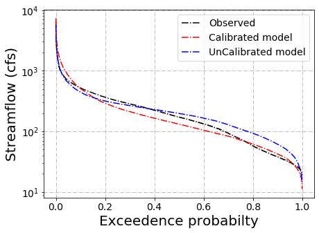
slope_Obs, slope_Calib, slope_UnCalib

(14.269005847953215, 14.863356580419119, 7.634983038137967)

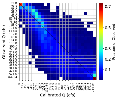
Time linked Flow Duration Curve (T-FDC)¶

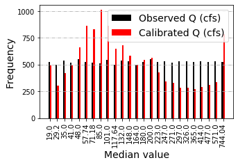
T-FDC is a confusion matrix analog based on binning. T-FDC tracks over and underestimation of a given day’s observed streamflow by the model depending on the bin it is located. The bins are defined based on observed streamflow with a user specified bin number. Thus, T-FDC is close to FDC but it has a time component as it tracks each timestep (e.g., daily). Thus, in performance evaluation, ideally, high number of occurrences (Frequency which is represented by hot colors in the heatmaps) needs to populate the diagonal - observed and predicted streamflow being in the same bin. That means, there is low over and unde-restimation of the hydrograph by the model.

The main function that plots T-FDC is timeLinkedFDC(.). It has inputs of:

observed and modeled streamflow.
Flag - is used to identify the binnig method with F=1 being Equal width, Flag=2 Equal Area, Flag=3 Equal Frequency binning.
Figure dimesions and titles.

binSize = 25
obs = CalibMat[:,0]
mod = CalibMat[:,4]
Flag = 3 # Binning method Equal 1 width, 2 Area, 3 depth (frequency) Frequency
ticks = [0,0.1,0.2, 0.3,0.5,0.7, 0.9]
diag = 1 # Number of diagonals [smaller better for Calibrated while larger 5 better for uncalibrated)

T_FDC = timeLinkedFDC(obs,diag, mod,binSize,Flag,[5,5], [5,3], 'Observed Q (cfs)', 'Calibrated Q (cfs)',
              ticks) #[7,7], [7.5,4]

binSize = 25
obs = UnCalibMat[:,0]
mod = UnCalibMat[:,4]
Flag = 3 # Binning method Equal 1 width, 2 Area, 3 depth (frequency) Frequency
ticks = [0,0.1,0.2, 0.3,0.5,0.7, 0.9]

T_FDC_Unc = timeLinkedFDC(obs,diag, mod,binSize,Flag,[5,5], [5,3], 'Observed Q (cfs)', 'Calibrated Q (cfs)',
              ticks) #[7,7], [7.5,4]

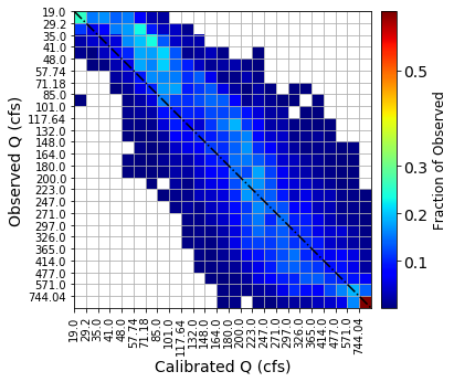
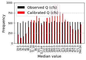
T_FDC , T_FDC_Unc

(0.3535625186415169, 0.33803317918700626)

Recession curves¶

Recession curves are imprints of the subsurface flow process. They capture the dynamics of streamflow as it is mostly driven by storage (absence of precipitation).

The main function plotting recession curves is plotRecession. It has inputs of:

ppt - precipitation data
Q - streamflow data
dateTime - timestamp
Season - For which season a recession curve is plotted. i. winter covers October to March (Note, this Months can be adjusted based on user preference in the source function) ii. Summer covers April to September (Note, this Months can be adjusted based on user preference in the source function) iii. All covers the entire year

plt.figure(figsize=[7,5]) #10,4, Winter, Summer, All
Season = 'Summer' #Winter, Summer, All
ReceCoeff_Obs = plotRecession(CalibMat[:,1], CalibMat[:,0],dateTimeD, 'Streamflow (Q) Recession','ko',
              'Observed',season = Season, alpha=1)
ReceCoeff_Calib = plotRecession(CalibMat[:,1], CalibMat[:,4],dateTimeD,'Streamflow (Q) Recession','ro',
              'Calibrated Model',season = Season,alpha=.5)
ReceCoeff_UnCalib = plotRecession(UnCalibMat[:,1], UnCalibMat[:,4],dateTimeD,'Streamflow (Q) Recession','bo',
              'UnCalibrated Model',season = Season,alpha=.5)

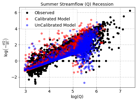
ReceCoeff_Obs, ReceCoeff_Calib, ReceCoeff_UnCalib

(array([ 1.38365002, -5.08668453]),
 array([ 1.39568974, -5.56100473]),
 array([ 1.17881136, -4.81572966]))

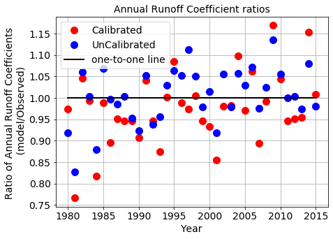
Water Balance¶

Annual Runoff coefficients (RC) are used as a signature measure of model’s capacity in capturing annual water balance. Compared to process networks (PN - section 7.2.2) that quantify information flow, RC quantfies how much mass is transfered from Precipitation to streamflow.

The main function in computaing RC is AnnualRunoffCoefficient(.) with the inputs of:

a table with precipitation, observed and model streamflow.
DateTime defining time stamp

tableCal = pd.DataFrame(data = CalibMat[:,(1,0,4)], columns=['basinPPT','ObsQ', 'ModelQ'],
                        index=dateTimeD)
tableUnCal = pd.DataFrame(data = UnCalibMat[:,(1,0,4)], columns=['basinPPT','ObsQ', 'ModelQ'],
                        index=dateTimeD)

# Compute annual and total runoff coefficients
Ann_CalR_obs, Tot_CalR_obs = AnnualRunoffCoefficient(tableCal,None,None,'basinPPT','ObsQ')
Ann_CalR_Mod, Tot_CalR_Mod = AnnualRunoffCoefficient(tableCal,None,None,'basinPPT','ModelQ')

Ann_UnCalR_obs, Tot_UnCalR_obs = AnnualRunoffCoefficient(tableUnCal,None,None,'basinPPT','ObsQ')
Ann_UnCalR_Mod, Tot_UnCalR_Mod = AnnualRunoffCoefficient(tableUnCal,None,None,'basinPPT','ModelQ')

plt.figure(figsize=[7,5])
plt.plot(Ann_CalR_Mod[:,0], Ann_CalR_Mod[:,1]/Ann_CalR_obs[:,1],'ro',label ='Calibrated',markersize=10)
plt.plot(Ann_UnCalR_Mod[:,0], Ann_UnCalR_Mod[:,1]/Ann_UnCalR_obs[:,1],'bo',label ='UnCalibrated',markersize=10)

plt.plot((np.min(Ann_CalR_obs[:,0]), np.max(Ann_CalR_obs[:,0])), 
         (1, 1),  linewidth=2, color='k', label='one-to-one line')
plt.xlabel('Year',fontsize=14)
plt.ylabel('Ratio of Annual Runoff Coefficients \n (model/Observed)',fontsize=14)
plt.title('Annual Runoff Coefficient ratios',fontsize=14)
plt.legend(fontsize=14)
plt.grid()
print(' Calibrated Runoff Coeffcient Ratio (modR/ObsR) =', np.round(Tot_CalR_Mod/Tot_CalR_obs,3),'\n',
      'Uncalibrated Runoff Coeffcient Ratio (modR/ObsR) = ', np.round(Tot_UnCalR_Mod/Tot_UnCalR_obs,3))

 Calibrated Runoff Coeffcient Ratio (modR/ObsR) = 0.969 
 Uncalibrated Runoff Coeffcient Ratio (modR/ObsR) =  1.003

Information theoretic based model benchmarking¶

Two model diagnostics are undertaken using information theoretic concepts. They are:

understanding the tradeoffs between predictive and functional model performances.
understanding model internal functions that lead to the predictive performance.

Achieving the above two undertakings, require computations of Mutual Information (MI) and Transfer Entropy (TE). While MI is used as a predictive performance metrics, TE is used as an indicator of model functional performance.

The computation of MI and TE requires different joint and marginal probabilities of the various flux and store hydrological variables referred in the input table header. In order to compute these probabilities, we used histogram based probability estimation.

Histogram based probabilities require defining:

the number of bins (nBins) used to develop the histogram,
how to handle higher and lower extreme values in the first and last bins of the histogram (low and high binPctlRange).

In order to understand the sensitivity of TE and MI to nBins and low and high binPctlRange, interactive widgets are used.

Hydrological time series are seasonal, e.g., seasonality driving both precipitation and streamflow. This seasonal signal may interfere with the actual information flow signal between two variables (e.g., information flow from precipitation to streamflow). As such, MI and TE values are sensitive to the seasonality of the hydrological time series (flux and store variables).In order remove the seasonal signal effect on MI and TE, this notebook computes MI and TE values based on the anomaly time series. The anomaly time series removes the seasonal signal of any store and flux variable by subtracting the long term mean of the day of the year average (DOY) from each time series measurement.

In computing the long term DOY average, ‘long term’ is a relative quantity - particularly in the face of non-stationarity. Therefore, we allow choosing different ‘long term’ time lengths in computing DOY. This choice can be set using the interactive widget (AnomalyLength).

In order to evaluate the statistical significance of MI and TE, we shuffle the flux and store variables repeatedly. For each repeated shuffle sample, we compute both TE and MI. Out of these repeated shuffle based MI and TE, we compute their 95 percentile as a statistical threshold (TE critical) to be surpassed by the actual MI and TE to be statistically significant. Here, as the 95% is sensitive to the number of repeated shuffles (nTests), we implemented interactive widget to understand this sensitivity.

We used interactive widgets to understand the sensitivity of TE/MI to these factors. These factors are abbreviated as follows.

nBins - the number of bins to be used in computing MI and TE
UpperPerct - upper percentile of the data to be binned
LowerPerct - lower percentile of the data to be binned
TransType - defines the options whether to perform MI and TE computation based on the anomaly time series or the raw data time series. Two options are implemented. (option 0 - raw data) and (option 1 - anomaly tranform)
AnomalyLength - length of ‘long term’ in computing DOY average for annomal time series generation.
nTests - the number of shuffles to be used in computing the 95% statistical threshold.

Executing the informtion theoretic code¶

In setting up the info-flow computation, the following basic info-theoretic options can be left to their default values. For understanding TE/MI sensitivity, please refer to the interactive widgets below.

optsHJ= {'SurrogateMethod': 2, # 0 no statistical testing, 1 use surrogates from file, 2 surrogates using shuffling, 3 IAAF method
        'NoDataCode': -9999,
        'anomalyPeriodInData' : 365 , # set it to 365 days in a year or 24 hours in a day #### 365days/year
        'anomalyMovingAveragePeriodNumber': 5, # how many years for computing mean for the anomaly ***
        'trimTheData' : 1,  #% Remove entire rows of data with at least 1 missing value? 0 = no, 1 = yes (default)
        'transformation' : 1 } # % 0 = apply no transformation (default), 1 = apply anomaly filter ***

# TE inputs 
optsHJ['doEntropy'] = 1
optsHJ['nTests'] = 100 # Number of surrogates (shuffles) to compute statistical significance (default = 300) ***
optsHJ['oneTailZ'] = 1.66
optsHJ['nBins'] = np.array([11]).astype(int) # ***
optsHJ['lagVect'] = np.arange(0,20) # lag days
optsHJ['SurrogateTestEachLag'] = 0
optsHJ['binType'] = 1 # 0 = don't do classification (or data are already classified), 1 = classify using locally bounded bins (default), 2 = classify using globally bounded bins
optsHJ['binPctlRange'] = [0, 99] # ***

# Input files and variable names
optsHJ['files'] =  ['./Data/'+nameFCalib] #nameFCalib #nameFunCalib
optsHJ['varSymbols'] = TableHeader
optsHJ['varUnits'] = TableHeader
optsHJ['varNames'] = TableHeader

# parallelization
optsHJ['parallelWorkers'] = 16 # parallelization on lags H and TE for each lag on each core.

# Saving results and preprocessed outputs
optsHJ['savePreProcessed'] = 0
optsHJ['preProcessedSuffix'] = '_preprocessed'
optsHJ['outDirectory'] = './Result/'
optsHJ['saveProcessNetwork'] = 1 
optsHJ['outFileProcessNetwork'] = 'Result'

# optsHJ['varNames']

# Define Plotting parameters
popts = {}
popts['testStatistic'] = 'TR' # Relative transfer intropy T/Hy
popts['vars'] = ['basin_ppt','model_Q'] # source followed by sink
popts['SigThresh'] = 'SigThreshTR' # significance test critical value
popts['fi'] = [0]
popts['ToVar'] = ['model_Q']
#popts

#ipywidgets
def WidgetInfoFlowMetricsCalculator(TransType, AnomalyLength, nTests, nBins, UpperPct, LowerPct):
    """ A widget helper function for CouplingAndInfoFlowPlot().
        CouplingAndInfoFlowPlot() is defined in the main file plottingUtilities_Widget.py
    """
    optsHJ['transformation'] = TransType
    optsHJ['anomalyMovingAveragePeriodNumber'] = AnomalyLength
    optsHJ['nTests'] = nTests
    optsHJ['nBins'] = np.array([nBins]).astype(int)
    optsHJ['binPctlRange'] = [LowerPct, UpperPct]
    
    
    CouplingAndInfoFlowPlot(optsHJ,popts) # calculates the information theoretic metrics (e.g. H, MI, TE)
                                          # and saves them in a pickle file. 

%%time
InfoFlowWidgetPlotter = ipywidgets.interactive( 
    WidgetInfoFlowMetricsCalculator, # as defined above
    
    TransType = ipywidgets.IntSlider(min=0, max=1, value=1),
    AnomalyLength = ipywidgets.IntSlider(min=0, max=10, value=5),
    nTests = ipywidgets.IntSlider(min=10, max=1000, value=10),
    nBins = ipywidgets.IntSlider(min=5, max=15, value=11),
    UpperPct = ipywidgets.IntSlider(min=90, max=100, value=99),
    LowerPct = ipywidgets.IntSlider(min=0, max=10, value=0) 
    

)
InfoFlowWidgetPlotter

Wall time: 77.7 ms

Below are the sensitivity analysis widgets. Please use the sliding widgets to interact with the different options and values

Interpreting the MI and TE results for model diagnostics¶

This section demonstrates the interpretation and use of the info-flow results to diagnose model performances in understanding the tradeoff between predictive and functional performance and revealing model internal functions in generating the predictive performance.

# Loading Info-flow Results for further Interpretation

RCalib = pd.read_pickle(r'./Result/Result_R.pkl')
optsHJCal = pd.read_pickle(r'./Result/Result_opts.pkl')

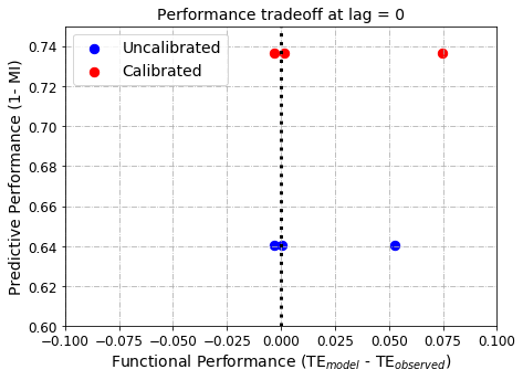
Tradeoff between functional and predictive model performances¶

Model development and parameter optimization can lead to tradeoffs between functional and predictive performances. In the figure below x-axis refers to model functional performance (the difference between observed and model information flow from input precipitation to output streamflow) while predictive model performance refers to the mutual information between observed and modeled streamflow.

The ideal model should have MI=1. (or 1-MI = 0) and TE_model - TE_observed = 0. As such, the (0,0) coordinate is the ideal model location.

In contrast,

a model in the right panel (TE_model - TE_observed > 0) is an overly deterministic model - i.e., a model that abstracts more information from input precipitation than the observed.
a model in the left panel (TE_model - TE_observed < 0) is a random model - i.e., a model that extracts poorly information from input precipitation compared to the observation.

As it is shown in the above TE/MI results, TE and MI are computed at different lags. The lags refer to the timestep by which the source variable is lagged in relation to the sink variable. The sink variable refers to model streamflow estimate (model_Q) while the remaining store/flux variable are source variables.

The interactive widget below offers an opportunity to understand the performance tradeoff of the model at the different lag timesteps.

%matplotlib inline
PerformanceTradeoff_widget = ipywidgets.interactive(
    plotPerformanceTradeoff,
    RCalib = fixed(RCalib),
    lag =ipywidgets.IntSlider(min=0, max=15, value=0),
    modelVersion = 'Calibrated', 
    WatershedName = 'Cedar River' , 
    SourceVar = ipywidgets.Dropdown(options=['basin_ppt', 'basin_tmin', 'basin_tmax'], disabled=False ) , 
    SinkVar = 'observed_Q',

)
PerformanceTradeoff_widget

# Plotting all in one functional and predictive performance metrics for precipitation, min and max air temperature.

plotPerformanceTradeoffNoFigure(0, RCalib, 'Calibrated', 'Cedar River','basin_ppt', 'observed_Q')

	Watershed	Functional Performance (TEmod - TEobs)	Predictive Performance (1-MI)
0	Cedar River	0.074643	0.736606

CalibTradOff = pd.DataFrame(np.nan, columns= ['Precipitation','Min Temperature','Max Temperature'],
            index = ['1-MI','TEmod - TEobs'])

# The numbers below are a result of executing the function: 
# plotPerformanceTradeoffNoFigure(0, RCalib, 'Calibrated', 'Cedar River','basin_tmin', 'observed_Q') as in the above cell.
# change the source variable and model versions to obtain all numbers.
CalibTradOff.iloc[0,:] = [0.736606,0.736606,0.736606] 
CalibTradOff.iloc[1,:] = [0.074643,-0.0033,0.001584]
CalibTradOff

	Precipitation	Min Temperature	Max Temperature
1-MI	0.736606	0.736606	0.736606
TEmod - TEobs	0.074643	-0.003300	0.001584

UnCalibTradOff = pd.DataFrame(np.nan, columns= ['Precipitation','Min Temperature','Max Temperature'],
            index = ['1-MI','TEmod - TEobs'])
UnCalibTradOff.iloc[0,:] = [0.64062,0.64062,0.64062]
UnCalibTradOff.iloc[1,:] = [0.05278, -0.003062,0.000258]
UnCalibTradOff

	Precipitation	Min Temperature	Max Temperature
1-MI	0.64062	0.640620	0.640620
TEmod - TEobs	0.05278	-0.003062	0.000258

plt.figure(figsize=[7,5])
Ms= 70
plt.scatter(UnCalibTradOff.iloc[1,:],UnCalibTradOff.iloc[0,:],s=Ms , color= 'b',label= 'Uncalibrated')
plt.scatter(CalibTradOff.iloc[1,:], CalibTradOff.iloc[0,:], s=Ms, color = 'r', label= 'Calibrated')

plt.axvline(x=0,color = 'k',ls=':', lw = 3)
plt.xlabel('Functional Performance (TE$_{model}$ - TE$_{observed}$)', size=14)
plt.ylabel('Predictive Performance (1- MI)', size = 14)
plt.grid(linestyle='-.')
plt.title('Performance tradeoff at lag = ' + str(0), size =14) 
plt.yticks(fontsize=12)
plt.xticks(fontsize=12)
plt.xlim([-0.1,0.1])
plt.ylim([0.6,0.75])
plt.legend(fontsize=14)
plt.show()

Process Network plots¶

Process Networks (PN) offer platform of presenting model internal functions based on transfer entropy. Similar to the above widgets, the process network plot below is generated at different lag timesteps. Please use the interactive widgets to reveal model internal ‘wiring’ at the different lags considered.

The PN variables and their direction are defined by the user depending on the availability of observations and expert knowledge.

def generateChordPlots(R,optLag,optsHJ,modelVersion):
    
    CalTR = R['TR'][0,optLag,:,:] # 0 file number, lags, from, to
    CalibChord = pd.DataFrame(data=CalTR, columns=optsHJ['varNames'], index=optsHJ['varNames'])
    
    # Excluding variables from PN plots.
    dfCal = CalibChord.drop(columns=['observed_Q'],index=['observed_Q'], axis=[0,1]) # 'basin_potet'
    
    # Set the diagonals to zero for the chord plot so that there is no self TE
    np.fill_diagonal(dfCal.values, 0) # no self TE
    
    # Rename Variable names for better plotting
    dfCal.columns = ['Precipitation','Min Temperature','Max Temperature','Streamflow','Soil Moisture','Snow melt','Actual ET', 'Potential ET']
    dfCal.index = ['Precipitation','Min Temperature','Max Temperature','Streamflow','Soil Moisture','Snow melt','Actual ET', 'Potential ET']
   
    # set exceptions based on physical principles
    dfCal.loc[:,'Min Temperature']=int(0)
    dfCal.loc[:,'Max Temperature']=int(0)
    dfCal.loc[:,'Precipitation']=int(0)
    dfCal.loc[('Streamflow'),:]=int(0)
    
    dfCal.loc[('Actual ET'),('Streamflow','Snow melt','Potential ET')]=int(0) # set all to 0?????
    dfCal.loc['Potential ET',('Streamflow','Snow melt')]=int(0)
    
    dfCal.loc['Soil Moisture','Snow melt']=int(0)
    dfCal.loc['Precipitation',('Actual ET','Potential ET')]=int(0)
    dfCal.loc['Snow melt',('Actual ET','Potential ET')]=int(0)
    
    
    
        # Calibrated chord diagram
    dataCal = hv.Dataset((list(dfCal.columns), list(dfCal.index), (dfCal.T*1000).astype(int)),
                  ['source', 'target'], 'value').dframe()
    
     # Now create your Chord diagram from the flattened data
    #plt.title('Uncalibrated')
    chord_Cal = hv.Chord(dataCal)
    chord_Cal.opts(title=modelVersion,
        node_color='index', edge_color='source', label_index='index', 
        cmap='Category10', edge_cmap='Category10', width=500, height=500)
    
    show(hv.render(chord_Cal) )
    print(dfCal)

def plot_widgetProcessNetworkChord(Lag):
    
    generateChordPlots(RCalib,Lag,optsHJ,'Calibrated') # lag=0 #str(nameFCalib)

PN_Chord_widget = ipywidgets.interactive(
        plot_widgetProcessNetworkChord,
   
    Lag = ipywidgets.IntSlider(min=0, max=15, value=0)
)
PN_Chord_widget

TOSSH and HydroBench interface¶

This section shows how to use the TOSSH toolbox in HydroBench. First, You need to have licence to matlab or use Octave. Second, you need to clone/download the Toolbox for Streamflow Signatures in Hydrology TOSSH toolbox to your working directory. Finally, follow the following steps to enable the Matlab and Python API.

How to Install MATLAB Engine API for Python: https://www.mathworks.com/help/matlab/matlab_external/install-the-matlab-engine-for-python.html

Setting up Matlab in Python:

python setup.py install # in the matlab rootfolder: i.e., cd “matlabroot\extern\engines\python”

Example on how to use a local function:

https://www.mathworks.com/help/matlab/matlab_external/call-user-script-and-function-from-python.html

import matlab.engine
eng = matlab.engine.start_matlab() # start matlab engine
# eng.quit() # end matlab engine

# Local Path to TOSSH functions.
# download/clone TOSSH and put it inside the main HydroBench directory
eng.addpath('./TOSSH-master/TOSSH_code/calculation_functions/');
eng.addpath('./TOSSH-master/TOSSH_code/signature_functions/');
eng.addpath('./TOSSH-master/TOSSH_code/utility_functions/');

Mat_DT = list(dateTimeD.strftime("%m/%d/%Y")) # Matlab datetime format

T_datetime = eng.datetime(list(Mat_DT),'InputFormat','MM/dd/yyyy') # as a datetime
T_datenum = eng.datenum(eng.datetime(list(Mat_DT),'InputFormat','MM/dd/yyyy')) # as a datenum

Q_mean = eng.sig_Q_mean(matlab.double(list(obs)),T_datenum)
Q_mean

248.15685604053513

Uncalibrated model Information flow analysis¶

Excercise For the uncalibrated model, please change the file name in section 7.1 as:

optsHJ['files'] =  ['./Data/'+nameFunCalib]

and rerun the subsequent cells.

Linking HydroBench and TOSSH

HydroBench - Hydrological Model Benchmarking and Diagnostic tool